This work is based on the work of Igor Bongoslavskyi .

ICP is an algorithm used to compute the rotation and the transformation ( rotation $R$ and translation $t$ ) between two sets of points, which target points $P = \{p_i\}$ and references points $Q = \{q_i\}$, where it uses and minimizes the differences of the two group of points. For example, ICP use in the 3D reconstruction point cloud or in 2D to match between scanning (for robot localizations)

In this projects I wrote a ICP using C++ and Eigne template. I used cv-Plot to show a visualization presentation of the points. CV-Plot is a library developed using purely opencv that can work in real time with easy integration.

ICP algorithms

In this project, I used different algorithms: (1) ICP based on SVD (2) ICP based on nonlinear least square.

First, I will start with SVD_ICP algorithms, where there are five steps to do the ICP which are.

Computer center data and transform them
Compute correspondences
Compute cross covariance matrix
Find $𝑅$ and $𝑡$ from SVD decomposition
Apply transformation and computer error

I will show the code and explain it for each step. However, before we start, it is essential to define the data type used in programming. So starting by defining the point, I use Eigen template Vector2d to store the value of the point $(x,y)$. And I used std::vectore to store the list of the point. Finally, I used Eigen::MatrixXd to process the rotation matrix and translation. Note: We need to keep the definition of variable constant using the Eigen library.

Computer center data and transform them

In this step we compute the mean center of all points in targets $\overline P=\frac{1}{n}\sum_{i=1}^n p_i$ and references $\overline Q=\frac{1}{n}\sum_{i=1}^n q_i$. After computing center of each point we reduce thier coordinate $p^{'} = p_i - \overline P$ and $q^{'} = q_i - \overline Q$.

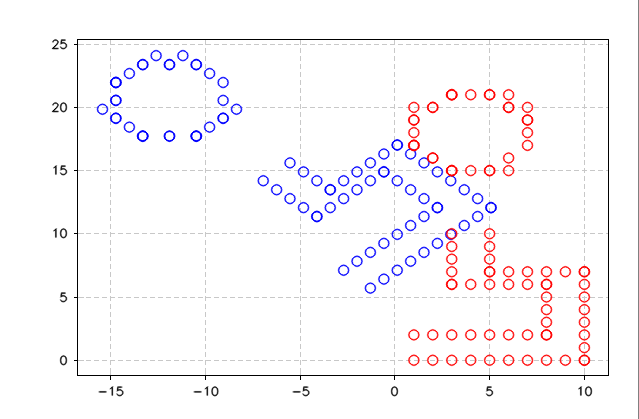
The data used to test this project is hand made data $Q$, then a transformation is applied to create the targets set $P$.

The function of computing the centre of the points is shown below. The input is a vector containing the list of points in Eigen::Vector2d format, and the output is Eigen::Vector2d as well.

Eigen::Vector2d Center_data(vector<Eigen::Vector2d> P)
{
	Eigen::Vector2d temp;
	temp << 0, 0;
	for (int i = 0; i < P.size(); i++)
	{
		temp += P[i];
	}
	temp = temp / P.size();
	return temp;
}

After computing the centre of data or the mean, we reduce the coordinate of the points using the following code.

for (int i = 0; i < Q.size(); i++)
	{
		Q_centered.push_back(Q[i] - center_of_Q);
	}

The output of transformation show below

We can see how the target points $P$ move to the center of refrence points $Q$.

Compute correspondences

We need to compute the correspondences between the target and reference points. At this point, there are many algorithms we can use to do the matching, such as search Tree and ANN. The name also knows correspondences algorithms or Registration algorithms. To measure the matched point, I will use linalg_norm to calculate the normal vector. The function is shown below, where the input is Vector2d, and the output is the difference.

double linalg_norm(Eigen::Vector2d p) {
	return sqrt(p(0) * p(0) + p(1) * p(1));
}

The correspondence algorithms consist of two loops where the first loop is to go through the point in reference point $Q$, and the second loop goes through the targets points $P$. Each point is measured using linalg_norm and compared with the minimum value. Then the index of both the target points and the reference points is stored in a vector. The function is shown below, where two vectors are the input and the output is a vector containing the matched indexes.

vector<Eigen::Vector2d> Get_correspondence_indices(vector<Eigen::Vector2d> P, vector<Eigen::Vector2d> Q)
{
	vector<Eigen::Vector2d> correspondences;
	for (int i = 0; i < P.size(); i++)
	{
		double min_distance = 99999999.9;
		int match_index = -1;
		for (int j = 0; j < Q.size(); j++)
		{
			double distance = linalg_norm(Q[j] - P[i]);
			if (distance < min_distance)
			{
				match_index = j;
				min_distance = distance;
			}
		}
		if (match_index != -1)
		{
			Eigen::Vector2d temp;
			temp << i, match_index;
			correspondences.push_back(temp);
		}
	}
	return correspondences;
}

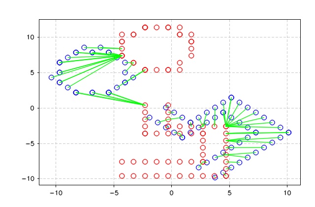
The figure below shows the output of the correspondences process, where each point from the reference points $Q$ is linked to the target points $P$. As can be seen, the matching process is not a great one, but it does the work for a 2D and minor points set.

Compute cross covariance matrix

Now we need to compute the cross covariance $K$ between the correspondeces points.

$$K=E[(q_i - \overline Q)(p_i - \overline P)^T)] $$ $$ =\frac{1}{N} \sum(q_i - \overline Q)(p_i - \overline P)^T) $$ $$ \approx \sum(q_i - \overline Q)(p_i - \overline P)^T) $$

The output of this equation $K$ will be a mratix of $2x2$, due to that $p_i , q_j \in \Bbb R^2$.

$$K = \begin{pmatrix}cov(p_{xi},q_{xj}) & cov(p_{xi},q_{yj})\\\ cov(p_{yi},q_{xj}) & cov(p_{yi},q_{yj})\end{pmatrix}$$

After computing the covariance, we will add $R$ and $t$ using Singular Value Decompositions SVD. SVD matrix is a factorization of the matrix. Where the output of SVD is three matrixes which $S$, $U$, and $T_V$. Therefore, $R=UV^T$ and $t=\mu_Q - R_{\mu_P}$. Using the Eigen library, we will compute the SVD of cov using Eigen::JacobiSVD; then, we compute the rotation and translation as shown in the below snap code.

// Step 4: Find  𝑅  and  𝑡  from SVD decomposition
Eigen::JacobiSVD<Eigen::MatrixXd> svd(cov, Eigen::ComputeFullU | Eigen::ComputeFullV);
auto R_found = svd.matrixU() * svd.matrixV().transpose();
auto T_found = center_of_Q - R_found * center_of_P;

Apply transformation and computer error

After getting the new $R$ and $t$, we need to apply the transformation to the target points $P$. Using the following function Apply_transform(). The function's output is a vector containing a list of corrected points. After that the Error is computed using linalg_norm function $E={\sqrt {P^{'} - Q} }$. Finally, we repeat the same step for few times until the error reaches the threshold. The function below is the ICP_SVD used. The function takes four inputs: two for reference points and target points. The vector takes the error at each iteration and the number of iterations.

vector<Eigen::Vector2d> ICP_svd(vector<Eigen::Vector2d> P, 
                                vector<Eigen::Vector2d> Q, 
                                vector<double>& error, 
                                int iterations = 10)
    {
        // Step 1: computer center data and transform them 
        Eigen::Vector2d center_of_Q = Center_data(Q);
        vector<Eigen::Vector2d> Q_centered;
        for (int i = 0; i < Q.size(); i++)
        {
            Q_centered.push_back(Q[i] - center_of_Q);
        }
        vector<Eigen::Vector2d> P_copy = P;
        // Start the loop
        for (int iter = 0; iter < iterations; iter++)
        {
            Plot_data(P_copy, Q);
    
            vector<Eigen::Vector2d> P_centered;
            Eigen::Vector2d center_of_P = Center_data(P_copy);
            for (int i = 0; i < P.size(); i++)
            {
                P_centered.push_back(P_copy[i] - center_of_P);
            }
    
            // Step 2: Compute correspondences
            auto correspondences = Get_correspondence_indices(P_centered, Q_centered);
    
            // Step 3: compute_cross_covariance
            auto cov = compute_cross_covariance(P_centered, Q_centered, correspondences);
    
            // Step 4: Find  𝑅  and  𝑡  from SVD decomposition
            Eigen::JacobiSVD<Eigen::MatrixXd> svd(cov, Eigen::ComputeFullU | Eigen::ComputeFullV);
            auto R_found = svd.matrixU() * svd.matrixV().transpose();
            auto T_found = center_of_Q - R_found * center_of_P;
    
            // Step 5: Apply transformation and computer error
            P_copy = Apply_transform(P_copy, R_found, T_found);
            double _error = Compute_Square_difference(P_copy, Q);
            error.push_back(_error);
            cout << "Squared diff: (P_corrected - Q) = " << _error << endl;
        }
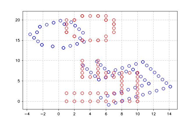
        Plot_data(P_copy, Q, 400);
        return P_copy;
    }

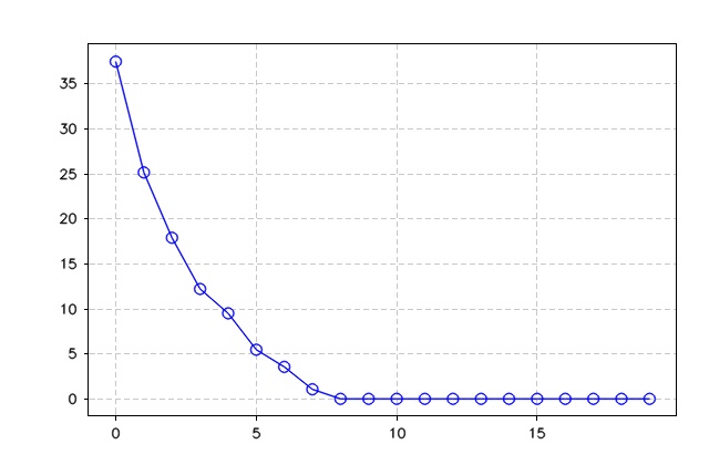
The figures below show the output of ICP_SVD algorithms and the error. As can be seen, the algorithm took seven iterations to drop the error to zero and match the two points sets.

ICP based on nonlinear least square

In this problem, we are working to reduce the error of the sum square distance between two points.

$$E = \sum[R*p_i + t - q_i]$$

$E$ is the value should be minimise by updating $R, t$. Keep note that $P$ is the only one update and due to the present of $R$ in the equation this function is non linear.

The minimizing problem starts with computing the corresponding point between both sets. We assume the pose is descripe as follow $\mathbf{x} = [x,y,\theta]^T$ where $\theta$ place in the the rotation matrix $R = \begin{pmatrix} cos(\theta) & -sin(\theta)\\\ sin(\theta) & cos(\theta)\end{pmatrix}$.

As shown above, we solve the problem of matching using SVD But other methods are more efficient. Instead of solving the SVD, we try to minimise the error between the corresponding points

$$ E = \sum_{i}[Rp_i + t - q_i]^2 $$

For the minimizing we update $R, t$ which will be represent in a vector $x=[x,y,\theta]^T$, where $R=\begin{pmatrix}cos(\theta) & -sin(\theta))\\\ sin(\theta) & -cos(\theta))\end{pmatrix}$ and $t = \begin{pmatrix} x \\\ y\end{pmatrix}$. We will keep updating the target points $p$ until they overlap on the reference point $Q$. Due to the presence of $R$, the problem becomes non-linear.

To solve this problem, we will use Gauss-Newton Method to minimise between the correspondence points. Therefore the error is the sum of the error between the correspondence points, shown in the equation below.

$$ e(x) = \sum_{i,j} e_{i,j}(x) $$

Keep in mind that $i,j$ refere to the correspondeces points between $P$ and $Q$ sets.

$$ e_{i,j}(x) = R_{\theta}p_i + t - q_j $$

Therefore, we need to minimize the error function $E(x)$.

$$ {min}_x \to {\sum_{i,j} ||R_{\theta}p_i + t - q_j||^2} $$

let $h_i(x) = R_{\theta}p_i + t$. The error function becom

$$ {min}_x \to {\sum_{i,j} ||h(x) - q_j||^2} $$

To compute the the local minimume value we will use Hessian matrix which is a square martix (n x n) of second-order partial derivative of a function see for more information

$$ H\Delta x = -E^{'} (x) $$

And $\Delta x\ = [\Delta x, \Delta, y, \Delta \theta]$ which represent the small change in $x$. Therefore the error function become

$$ E^{'}(x) = J(x)e(x) $$

$J(x)$ is the jacobian and it show below

$$ J = \begin{pmatrix}1 & 0 & -sin(\theta){p_i}^x-cos(\theta){p_i}^y)\\\ 0 & 1 & cos(\theta){p_i}^x-sin(\theta){p_i}^y)\end{pmatrix} $$

The code below shows a function that creates the jacobian using Eigen::MatrixXd that generate a matrix size (2x3).

Eigen::MatrixXd Jacobian(Eigen::Vector3d _x, Eigen::Vector2d point)
{
	double angle = _x(2);
	double x = point(0);
	double y = point(1);
	Eigen::MatrixXd J(2, 3);
	J << 1, 0, -sin(angle) * x - cos(angle) * y,
		0, 1, cos(angle)* x - sin(angle) * y;

	return J;
}

Eigen::Vector2d Error(Eigen::Vector3d x, Eigen::Vector2d p, Eigen::Vector2d q)
{
	auto rotation = Get_R(x(2));
	Eigen::Vector2d translation;
	translation << x(0), x(1);
	auto prediction = rotation * p - translation;
	return (prediction - q);
}

Now we can solve Hessian $H = \begin{pmatrix} 0 & 0& 0\\\ 0 & 0& 0\\\ 0 & 0& 0 \end{pmatrix}$ and $g =\begin{pmatrix} 0 \\\ 0 \\\ 0 \end{pmatrix}$. Therefore to solve the system we create a function call Prepare_system to compute Hessian matrix.

The function Prepare_system take seven inputs which are $x$, Point set $P$ and $) Q$, the correspondences index vectors, H matrix, g vector and the error chi. The last three variables were updated and returned using pass by reference.

The function loop on all correspondence points to compute the Jacobian, then update the H and g. Where $H= J^T J$ and $g=J^T e$. Note that the $weight$ eliminates the outlier point above the threshold.

void Prepare_system(Eigen::Vector3d x,
	vector<Eigen::Vector2d> P,
	vector<Eigen::Vector2d> Q,
	vector<Eigen::Vector2d> correspondences,
	Eigen::MatrixXd& H,
	Eigen::Vector3d& g,
	double& chi)
{
	for (int i = 0; i < correspondences.size(); i++)
	{
		auto p_point = P[correspondences[i](0)];
		auto q_point = Q[correspondences[i](1)];
		auto e = Error(x, p_point, q_point);
		double weight = Kernal(10, e);
		auto J = Jacobian(x, p_point);
		H += weight * J.transpose() * J;
		g += weight * J.transpose() * e;
		chi += e.transpose() * e;
	}
}

ICP non-linear Least Square

ICP based on non-linear least-square has four steps which are shown in the code below. The first step is to initialize the for loop for the limited iteration. Then we initialize the x vector that contains the translation and $\theta$. Also, Hessian matrix $H$ and $g$ initilized with zeros.

We start processing the point by computing the corresponding point using the defined function. Next, we pass the data to the Prepare_system function to compute Hessain matrix $H$ and $g$. Using $H$ and $g$, we solve the equation using the Eigen inbuild function. bdcSvd . the output of bdcSvd $\delta x$ is the small motion computed between the both points group.

Using $\delta x$ to update the overall $x$ and then computer $R$ and $t$. The target point then updated using the descibe function Apply_transform and the final translation and rotation is updated as well using $R_{final} = R * R_{final}$ and $T_{final} += t$.

Note that we use chi as a threshold where it stop when it reach below a certine value.

vector<Eigen::Vector2d> ICP_least_squares(vector<Eigen::Vector2d> P, 
										  vector<Eigen::Vector2d> Q, 
										  vector<double>& error, 
										  int iterations = 10)
{
	Eigen::MatrixXd R_final = Eigen::MatrixXd::Identity(2, 2);
	Eigen::Vector2d T_final = Eigen::Vector2d::Zero();
	vector<Eigen::Vector2d> P_copy = P;
	for (int i = 0; i < iterations; i++)
	{
		Plot_data(P_copy, Q, 80);
		Eigen::Vector3d x = Eigen::Vector3d::Zero();
		Eigen::MatrixXd rot = Get_R(x(2));
		Eigen::Vector2d t;
		t(0) = x(0);
		t(1) = x(1);
		Eigen::MatrixXd H = Eigen::MatrixXd::Zero(3, 3);
		Eigen::Vector3d g = Eigen::Vector3d::Zero(3);
		double chi = 0.0;
		// step 1: compute correspondese 
		auto correspondences = Get_correspondence_indices(P_copy, Q);

		// step 2: compute H, g and Chi
		Prepare_system(x, P_copy, Q, correspondences, H, g, chi);
		error.push_back(chi);
		// Step 3: solve the linear equation
		Eigen::Vector3d dx = -1 * H.bdcSvd(Eigen::ComputeThinU | Eigen::ComputeThinV).solve(g);

		// step 4: update x and apply transformation
		x += dx;
		x(2) = atan2(sin(x(2)), cos(x(2)));
		rot = Get_R(x(2));
		t(0) = x(0);
		t(1) = x(1);
		P_copy = Apply_transform(P_copy, rot, t);
		R_final = rot * R_final;
		T_final += t;
		if (chi < 0.0001)
		{
			break;
		}
	}
	return P_copy;
}

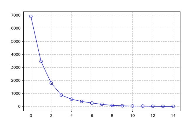
The figure below shows the output of ICP least square and the error output.

For the full code check this link Guthub_code

Refrences

Srinath Rajagopalan

Link_1

and the explination of Cyrill Stachniss

Jyoti Sunkara

M. Greenspan and M. Yurick, "Approximate k-d tree search for efficient ICP," Fourth International Conference on 3-D Digital Imaging and Modeling, 2003. 3DIM 2003. Proceedings., 2003, pp. 442-448, doi: 10.1109/IM.2003.1240280.

2D Iterative Closest Point (ICP)

ICP using c++ and eigen library